
Review the key concepts, formulae, and examples before starting your quiz.
🔑Concepts
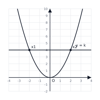
To solve an equation of the form graphically, you identify the -coordinates where the curve intersects the horizontal line . These intersection points represent the solutions or 'roots' of the equation.
To solve , plot both functions on the same axes. The solutions are the -coordinates of the points where the two graphs intersect. For example, to solve , find where the cubic curve meets the straight line.
If a curve is already drawn and you need to solve a modified equation , rearrange the new equation until one side matches the existing graph. The other side tells you which straight line must be drawn to find the solutions.
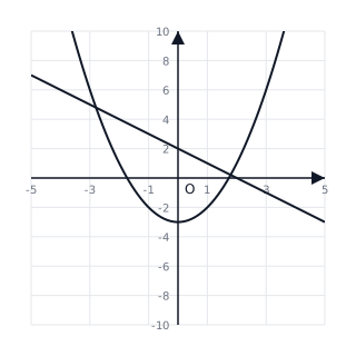
The gradient of a curve at a specific point is found by drawing a tangent to the curve at that point. The gradient of this straight line is calculated using , providing the instantaneous rate of change.
📐Formulae
(Equation of the straight line to be drawn)
(Gradient calculation for a tangent line)
(Standard quadratic to be solved via intercepts)
💡Examples
Problem 1:
The graph of is already drawn. Use the graph to solve the equation .
Solution:
- Rearrange the target equation to match the graph: .
- This becomes .
- Draw the horizontal line on the same axes as the curve.
- Identify the x-coordinates where the line intersects the curve .
- Solutions are and .
Explanation:
To use an existing graph to solve a new equation, we must manipulate the new equation until one side is identical to . The other side of the equation tells us what additional line or curve needs to be drawn.
Problem 2:
Estimate the gradient of the curve at the point where .
Solution:
- Locate the point on the graph of .
- Use a ruler to draw a tangent line that just touches the curve at this point.
- Pick two points on this tangent line, e.g., and .
- Calculate .
- The estimated gradient is 9.
Explanation:
The gradient of a curve changes at every point. A tangent line represents the instantaneous rate of change at that specific point. Accuracy depends on the precision of the drawn tangent.
Problem 3:
Find the range of values of for which the equation has no real solutions.
Solution:
- Observe the vertex (minimum point) of the parabola .
- The vertex is at .
- -value at vertex: .
- If the line is below the minimum point, there are no intersections.
- Therefore, .
Explanation:
Graphically, 'no real solutions' means the line does not intersect the curve . For a U-shaped quadratic, this occurs when is less than the minimum -value.
Problem 4:
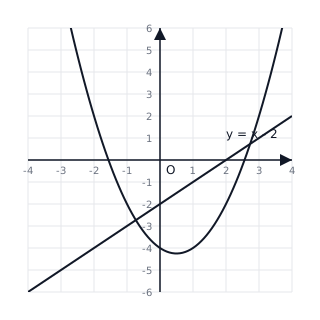
The diagram shows the graph of . By drawing a suitable straight line, solve the equation .
Solution:
- Start with the equation to solve:
- Rearrange it to make one side look like the plotted graph ():
- This means we must draw the line on the grid.
- The intersection points of and are at and .
Explanation:
To use an existing graph to solve a different equation, we manipulate the target equation so that the LHS is identical to the function already drawn. The resulting RHS is the equation of the line that needs to be plotted.
Problem 5:
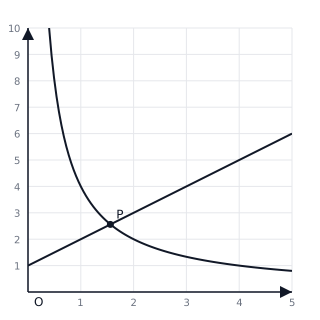
Solve the simultaneous equations and graphically for .
Solution:
- Plot the reciprocal graph for positive values of .
- Plot the linear graph .
- Locate the point of intersection in the first quadrant.
- The graphs intersect at approximately. Therefore, .
Explanation:
Simultaneous equations are solved graphically by finding the coordinates where the two graphs meet. For , we only look at the intersection in the first quadrant.