
Linear Programming - Introduction, related terminology (constraints, objective function, optimization)
Review the key concepts, formulae, and examples before starting your quiz.
🔑Concepts
Linear Programming Problem (LPP) is an optimization method used to find the maximum or minimum value of a linear function, called the Objective Function, subject to a set of linear inequalities called constraints. The variables and are known as decision variables.

The Feasible Region is the set of all points that satisfy all given constraints simultaneously. If the region is enclosed by lines on all sides, it is called Bounded; if it extends infinitely in any direction, it is Unbounded.
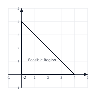
Corner Point Theorem: The optimal value (maximum or minimum) of the objective function , if it exists, must occur at one of the corner points (vertices) of the feasible region.
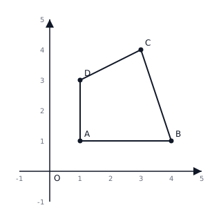
Non-negativity constraints restrict the feasible region to the first quadrant of the Cartesian plane, representing physical quantities that cannot be negative (e.g., number of items produced).
📐Formulae
Objective Function:
General Linear Constraint:
Non-negativity Constraints:
Condition for Bounded Region: and exist at corner points.
Condition for Unbounded Region: If the region is unbounded, a maximum or minimum may or may not exist.
💡Examples
Problem 1:
Maximize subject to the constraints: , , .
Solution:
- Convert the inequality to an equation: . The line passes through and .
- Since the constraint is , the feasible region is the area below the line in the first quadrant (due to ).
- The corner points of the feasible region are , , and .
- Evaluate at each corner point:
- At
- At
- At
- Comparing the values, the maximum value of is at the point .
Explanation:
The problem asks for the maximum value of a linear function. By plotting the boundary and identifying the vertices of the resulting triangle (feasible region), we test each vertex in the objective function to find the highest value.
Problem 2:
Minimize subject to: , , .
Solution:
- Plot the boundary lines: (intercepts ) and (intercepts ).
- The constraints are 'greater than or equal to', so the feasible region is the area above both lines in the first quadrant (unbounded region).
- Find the corner points of the feasible region: and . Note that the intersection of the two lines is at .
- Evaluate at the corner points:
- At
- At
- Since the value is the same at both points, any point on the line segment joining and that satisfies the constraints will give the minimum value of .
Explanation:
This example demonstrates a minimization problem with an unbounded feasible region. It also shows a special case where multiple points (an entire line segment) provide the same optimal value.
Problem 3:
Minimize subject to , , .
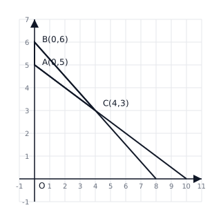
Solution:
- Identify corner points by solving boundary equations:
- Line 1: . Intercepts are and .
- Line 2: . Intercepts are and .
- Intersection of and : Multiply Line 1 by 2: . Subtract from Line 2: . Substitute in Line 1: .
- Corner points of feasible region: , , .
- Evaluate at corners:
- At
- At
- At Minimum value is 2300 at .
Explanation:
The feasible region is the small triangular area bounded by the -axis and the two intersecting lines. The minimum occurs at the intersection point because it has the lowest cost coefficient weight.
Problem 4:
Find the maximum value of subject to , , .
Solution:
- Analyze constraints:
- Constraint 1:
- Constraint 2:
- Check for common region:
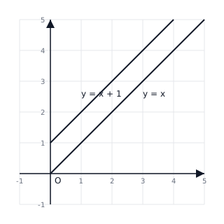
- The first inequality represents the region above the line .
- The second inequality represents the region below the line .
- Since the lines and are parallel and the required regions are in opposite directions, there is no point that satisfies both conditions simultaneously.
- Therefore, the feasible region is empty.
Explanation:
When constraints are contradictory, no feasible region exists. In such cases, the LPP has no optimal solution.