
Review the key concepts, formulae, and examples before starting your quiz.
🔑Concepts
The Feasible Region is the set of all points that satisfy all given linear constraints simultaneously, including the non-negativity constraints . This region is usually a convex polygon.
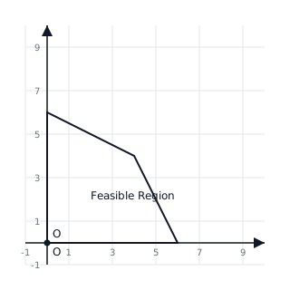
The Corner Point Theorem states that the optimal value (maximum or minimum) of the objective function , if it exists, must occur at one of the vertices (corner points) of the feasible region.
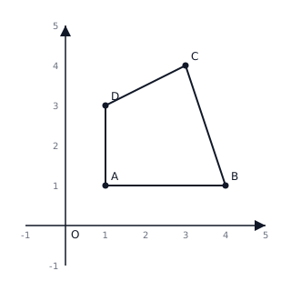
Constraints of the form usually represent a half-plane containing the origin (if ), while represents the half-plane away from the origin.
Iso-profit or Iso-cost lines: These are lines where the objective function has a constant value. Moving these lines parallel to themselves helps identify the 'last' point of contact with the feasible region, indicating the optimum.
📐Formulae
General form of Objective Function:
General form of Linear Constraints: or
Non-negativity constraints:
Equation of a boundary line:
Slope-intercept form for plotting lines:
💡Examples
Problem 1:
Maximize subject to the constraints: , , and .
Solution:
Step 1: Convert inequalities to equations to find intercepts. For : When ; When . For : When ; When .
Step 2: Plot the lines and find the feasible region. Since both constraints are , the region is towards the origin. The non-negativity constraints limit the region to the first quadrant.
Step 3: Find the intersection point of and . Multiplying the first by 2 and the second by 5: Subtracting: Substitute : .
Step 4: Evaluate at corner points:
- At
- At
- At
- At
Maximum value of is at .
Explanation:
We first identify the boundary lines and shade the region satisfied by all inequalities. The feasible region is a quadrilateral with vertices and . We then test the objective function at each vertex to find the maximum value.
Problem 2:
Minimize subject to .
Solution:
Step 1: Find intercepts for boundary lines. Line 1: and . Line 2: and .
Step 2: Identify the Feasible Region. Since constraints are , the region is 'unbounded' and away from the origin (above the lines).
Step 3: Find the corner points of the unbounded region.
- Intersection of and the y-axis: (since is higher than ).
- Intersection of the two lines: (Line 1 multiplied by 2) Subtracting: . Substituting : . Corner point: .
- Intersection of and the x-axis: (since is further right than ).
Step 4: Evaluate at corner points:
- At
- At
- At
Minimum value of is at .
Explanation:
In this minimization problem with constraints, the feasible region is unbounded in the first quadrant. The corner points are and . After testing these points, we find the minimum value at .
Problem 3:
Maximize subject to: , , .
Solution:
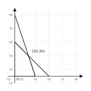
- Plot lines: (intercepts ) and (intercepts ).
- Identify Feasible Region vertices by solving equations:
- Intersection of and : Subtraction gives . Vertex is .
- Other vertices: .
- Evaluate at vertices:
- At
- At
- At
- At Max value is 120 at .
Explanation:
We identify the corner points of the shaded region bounded by the two lines and the axes. The maximum value of the linear function is found by testing each corner point.
Problem 4:
Minimize subject to , , .
Solution:
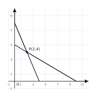
- Plot boundary lines: (intercepts ) and (intercepts ).
- The region is unbounded 'above' the lines.
- Solve for intersection: . Subtract . Then . Intersection is .
- Vertices: .
- Evaluate :
- At
- At
- At Minimum value is 26 at .
Explanation:
Since the inequalities are , the feasible region is the area above and to the right of the boundary lines. The minimum occurs at the vertex closest to the origin.