
Review the key concepts, formulae, and examples before starting your quiz.
🔑Concepts
The objective function represents the quantity to be maximized or minimized. In a graphical representation, the iso-profit or iso-cost lines move parallel to each other as the value of changes.
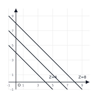
Constraints are linear inequalities that define the feasible region. Non-negativity constraints restrict the solution to the first quadrant.
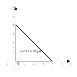
The Corner Point Theorem states that the optimal (maximum or minimum) value of the objective function occurs at one of the vertices (corner points) of the feasible region.
A bounded feasible region is a closed polygon, ensuring both a maximum and a minimum exist. An unbounded feasible region may not have a maximum value if the region extends infinitely in the direction of increasing .
📐Formulae
General Objective Function:
Linear Inequality Constraint: or
Non-negativity Conditions:
Slope of the Objective Function Line:
Intersection Point of two lines and found using simultaneous equations.
💡Examples
Problem 1:
Maximize subject to the constraints: , , .
Solution:
- Identify the Boundary Lines:
- (passes through and )
- (passes through and )
-
Find the Intersection Point of and : \nSubtract from : . \nSubstitute into . \nIntersection Point: .
-
Determine the Feasible Region: \nSince both constraints are , the region is toward the origin. The vertices of the bounded feasible region are:
- (from )
- (Intersection)
- (from )
- Evaluate the Objective Function at each vertex:
- At
- At
- At
- At
- Conclusion: \nThe maximum value of is , which occurs at the point .
Explanation:
We use the Corner Point Method by first sketching the linear equations on a graph to find the feasible region in the first quadrant. By calculating at every vertex of this region, we identify the highest value as the optimal solution.
Problem 2:
Minimize subject to: , , .
Solution:
- Identify the Boundary Lines:
- (Intersects axes at and )
- (Intersects axes at and )
-
Find the Intersection Point: \nMultiply by : . \nSubtract this from : . \nSubstitute into : . \nIntersection Point: .
-
Determine the Feasible Region: \nSince both constraints are , the region is 'Unbounded' and away from the origin. Vertices are:
- Evaluate :
- At
- At
- At
- Conclusion: \nThe minimum value of is at the point .
Explanation:
For minimization with constraints, the feasible region is typically unbounded away from the origin. We identify the 'outer' corner points and evaluate the cost function to find the minimum value.
Problem 3:
Maximize subject to the constraints: , , .
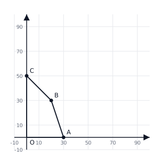
Solution:
- Plot the lines and .
- Identify the feasible region bounded by the axes and these lines.
- Find corner points: , , (intersection of both lines), and .
- Evaluate at each point:
- At
- At
- At
- At
Max value is 120 at .
Explanation:
The maximum value is found by testing all vertices of the convex polygon formed by the constraints. The point yields the highest .
Problem 4:
Minimize subject to: , , .
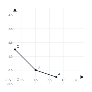
Solution:
- Plot and .
- The feasible region is unbounded and lies above/right of the lines.
- Corner points: , , and .
- Evaluate :
- At
- At
- At
Minimum value is 7 at .
Explanation:
For an unbounded region, we find the minimum at the corner points. Since the coefficients of are positive and the region is restricted to the first quadrant, a minimum exists.